Gradients of GAN Objectives

Mar 8, 2021

This technical post will offer a new view of common training objectives for generative adversarial networks (GANs), including a justification for the widely-used non-saturating loss.

The gradient of the discriminator

First, let’s look at the original GAN loss function and show that it’s simpler than it looks. As defined in Goodfellow et al. (2014), it’s

$L(G, D) = \mathbb{E}_{x \sim p_\text{data}(x)}[\log D(x)] + \mathbb{E}_{z \sim p_z(z)}[\log(1 - D(G(z)))]$

where $p_\text{data}(x)$ is the data distribution, $p_z(z)$ is the noise distribution, $D(x)$ is the discriminator, and $G(z)$ is the generator.

To analyze this loss function, we’ll use the same idea as in my post on the cross entropy loss: instead of looking at the function itself, we’ll look at its gradient.

We’ll assume the discriminator uses the standard method of obtaining the output probability $D(x)$ by applying the logistic sigmoid function to a scalar output $\ell$ :

$D(x) = \frac{e^\ell}{1 + e^\ell}$

Taking the logarithm:

$\log D(x) = \ell - \log(1 + e^\ell)$

And the derivative:

$\begin{align*} \frac{\text{d}}{\text{d}\ell}[\log D(x)] &= \frac{\text{d}}{\text{d}\ell}[\ell - \log(1 + e^\ell)] \\ &= 1 - \frac{e^\ell}{1 + e^\ell} \\ &= 1 - D(x) \end{align*}$

This is quite surprising: by taking the derivative of $\log D(x)$ with respect to $\ell$ , we get exactly $1 - D(x)$ , the probability that the discriminator thinks $x$ is fake.

We can do the same calculation for the flipped probability $\log(1 - D(x))$ :

$\begin{align*} \frac{\text{d}}{\text{d}\ell}[\log(1 - D(x))] &= \frac{\text{d}}{\text{d}\ell}\left[\log\left(\frac{1}{1+e^\ell}\right)\right] \\ &= \frac{\text{d}}{\text{d}\ell}[-\log(1 + e^\ell)] \\ &= -\frac{e^\ell}{1 + e^\ell} \\ &= -D(x) \end{align*}$

We’re going to use these facts to analyze the discriminator loss function $L(G, D)$ .

First, some change of notation: let’s write $\ell$ as $\ell(x)$ to make it clear what input produced $\ell$ . And let’s define $g(x) = \nabla_\theta(\ell(x))$ , where $\theta$ represents the parameters of the discriminator. The motivation for this definition of $g(x)$ is that it will let us write the full gradient $\nabla_\theta[f(D(x))]$ as the product $g(x) \cdot \frac{\text{d}}{\text{d}\ell}[f(D(x))]$ , where either $f(x)=\log x$ or $f(x)=\log(1-x)$ .

Now we can write the gradient of $L(G, D)$ as follows:

$\begin{align*} &\nabla_\theta \, L(G, D) \\ &= \nabla_\theta\left[ \mathbb{E}_{x \sim p_\text{data}(x)}[\log D(x)] + \mathbb{E}_{z \sim p_z(z)}[\log(1 - D(G(z)))] \right] \\ &= \mathbb{E}_{x \sim p_\text{data}(x)}[\nabla_\theta \log D(x)] + \mathbb{E}_{z \sim p_z(z)}[\nabla_\theta \log(1 - D(G(z)))] \\ &= \mathbb{E}_{x \sim p_\text{data}(x)}[g(x) \cdot (1 - D(x))] + \mathbb{E}_{z \sim p_z(z)}[g(G(z)) \cdot (-D(G(z))) ] \\ &= \mathbb{E}_{x \sim p_\text{data}(x)}[g(x) \cdot (1 - D(x))] - \mathbb{E}_{z \sim p_z(z)}[g(G(z)) \cdot D(G(z)) ] \\ &= \hspace{1.05em} \mathbb{E}_{x \sim p_\text{data}(x)}[g(x) \cdot \text{Pr}(x\text{ is misclassified})] \\ &\hspace{1.2em} - \mathbb{E}_{z \sim p_z(z)}[g(G(z)) \cdot \text{Pr}(G(z)\text{ is misclassified}) ] \hspace{3em} (*) \end{align*}$

This gives a clearer view of the GAN objective than looking at the original loss function. From this, we see that the discriminator’s goal is simply to increase $\ell(x)$ for real inputs and decrease $\ell(x)$ for fake inputs, with the caveat that inputs are weighted by their probability of being misclassified.

This is an example of a general principle in machine learning, which is that learning algorithms should focus on examples the model gets wrong over examples the model gets right. Other examples of this principle include:

The perceptron learning algorithm, which only updates on mistakes.
The hinge loss, which has no gradient when the prediction $y$ has the right sign and $|y| > 1$ .
Logistic regression, which has the same loss function as a GAN discriminator.

The non-saturating loss

If we accept the principle that a model should weight its mistakes more than its successes, then there’s something not quite right about $(*)$ . Though $(*)$ matches this principle when used for the discriminator, it’s quite the opposite for the generator. From the perspective of the generator, the examples which are misclassified by the discriminator are successes, not mistakes. Applying this principle to the training of the generator would suggest that we should weight more heavily the examples which are correctly classified by the discriminator. In fact, this is exactly what is done in practice. From Goodfellow et al. (2014):

In practice, equation 1 [the loss function which $(*)$ is the gradient of] may not provide sufficient gradient for $G$ to learn well. Early in training, when $G$ is poor, $D$ can reject samples with high confidence because they are clearly different from the training data. In this case, $\log(1 - D(G(z)))$ saturates. Rather than training $G$ to minimize $\log(1 - D(G(z)))$ we can train $G$ to maximize $\log D(G(z))$ . This objective function results in the same fixed point of the dynamics of $G$ and $D$ but provides much stronger gradients early in learning.

Though Goodfellow et al. motivate it differently, referring to vanishing gradients early in training, the idea is precisely the same: maximizing $\log D(G(z))$ leads to weighting $g(x)$ by the probability that $x$ is correctly classified by the discriminator. This is called the non-saturating loss and it is used ubiquitously, for example in StyleGAN 2 (Karras et al., 2020).

The hinge loss

The hinge loss has a long history, but its use in GANs dates to Lim and Ye (2017) and Tran et al. (2017). It was used in SAGAN (Zhang et al., 2018) and BigGAN (Brock et al., 2018).

Like the non-saturating loss, it uses different loss functions for the generator and the discriminator:

$\begin{align*} L_D &= -\mathbb{E}_{x \sim p_\text{data}(x)}[\min(0, -1 + D(x))] - \mathbb{E}_{z \sim p_z(z)}[\min(0, -1 - D(G(z)))] \\ L_G &= -\mathbb{E}_{z \sim p_z(z)}[D(G(z))] \end{align*}$

The gradient of this loss is similar to the gradient in $(*)$ . In this context we’ll define $g(x) = \nabla_\theta[D(x)]$ , since $D(x)$ here is the analogue of $\ell(x)$ previously. The gradient of the discriminator is:

$\begin{align*} -\nabla_\theta \, L_D &= \hspace{1.05em} \mathbb{E}_{x \sim p_\text{data}(x)} \left[ \begin{cases} g(x) & \text{if $D(x) < 1$} \\ 0 &\text{otherwise} \end{cases}\right] \\ &\hspace{1.2em} - \mathbb{E}_{z \sim p_z(z)}\left[ \begin{cases} g(G(z)) &\text{if $D(G(z)) > -1$} \\ 0 &\text{otherwise} \end{cases} \right] \end{align*}$

You can see the similarity to $(*)$ : the discriminator gets no gradient from examples where its prediction is correct and has absolute value greater than 1. This serves the same purpose as weighting by misclassification probability in $(*)$ : it prevents the discriminator from continuing to focus on examples it already gets right.

You can also see why it’s necessary to use a different loss function for the generator. Otherwise, the generator would get no gradient from examples the discriminator confidently classifies as fake, which is precisely the opposite of what we want.

You might ask whether the reasoning from the previous section on the non-saturating loss can also be applied here. In fact, there is a direct analogue of the non-saturating loss:

$L_G = -\mathbb{E}_{z \sim p_z(z)}[\min(0, -1 + D(G(z)))]$

This cuts off the gradient using the same rule as $L_D$ , but when $D(G(z)) > 1$ rather than when $D(G(z)) < -1$ . As I mentioned in the previous section on the non-saturating loss, this is justified by the principle that learning algorithms should focus on their mistakes over their successes, since from the generator’s perspective, the mistakes are the cases where $D(G(z)) < 0$ .

I’m not aware of anyone using this alternate loss. If you’ve tried it, let me know.

Adding a W

Now let’s consider the Wasserstein GAN (Arjovsky et al., 2017). WGAN can be obtained from the original GAN by making the following modifications:

Stop weighting $g(x)$ by the probability of $x$ being misclassified. Instead, weight all $g(x)$ equally.
Enforce a Lipschitz constraint on $\theta$ .

In the original paper, WGAN is presented differently. Arjovsky et al. motivate it by arguing that we should minimize the Wasserstein distance between the data distribution and the generator distribution, then proposing to use an alternative representation of the Wasserstein distance to approximate it using the discriminator. However, I prefer this presentation because it makes it clear that WGAN is very similar to the original GAN.

Why is my formulation of WGAN equivalent to that of Arjovsky et al.? Their formulation is to learn a discriminator $f(x)$ . As in the section on the hinge loss, in this context I’ll define $g(x) = \nabla_\theta \, f(x)$ , since $f(x)$ is the analogue of $\ell(x)$ previously. The objective for their discriminator is to maximize

$\mathbb{E}_{x \sim p_\text{data}(x)}[f(x)] - \mathbb{E}_{z \sim p_z(z)}[f(G(z))]$

and the gradient of this quantity is

$\mathbb{E}_{x \sim p_\text{data}(x)}[g(x)] - \mathbb{E}_{z \sim p_z(z)}[g(G(z))]$

which is equal to $(*)$ without the weighting by misclassification probability.

Why does WGAN add the Lipschitz constraint? This was motivated in the WGAN paper by the fact that a Lipschitz constraint is necessary to estimate the Wasserstein distance — specifically, if the Wasserstein distance between $p$ and $q$ is $d$ , then an optimal discriminator $f(x)$ between $p$ and $q$ constrained to have Lipschitz constant $L$ will satisfy: $\mathbb{E}_{x \sim p(x)}[f(x)] - \mathbb{E}_{x \sim q(x)}[f(x)] = L \cdot d.$

But there’s another way to look at the Lipschitz constraint: we can view it as a regularizer on the discriminator that keeps its gradients bounded and makes the generator easier to optimize. This view is supported by Kurach et al. (2019), which found that spectral normalization, a common way of enforcing the Lipschitz constraint (Miyato et al., 2018), helped all GAN variants in their study, not just WGAN:

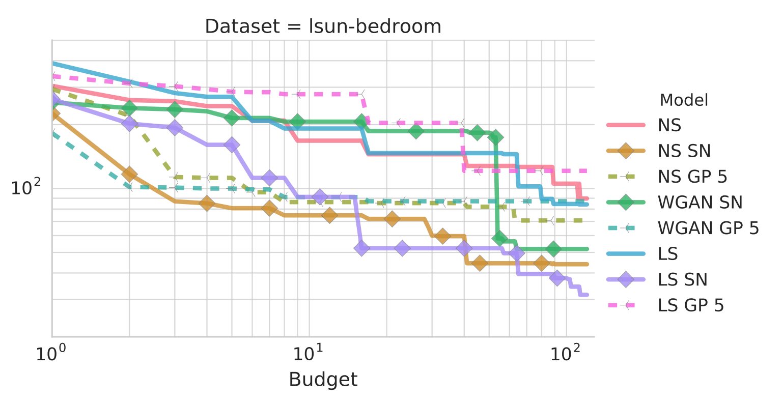
Subplot of Figure 2 from Kurach et al. (2019). NS means non-saturating loss, LS means least-squares loss, SN means spectral normalization, GP means gradient penalty (another way of enforcing the Lipschitz constraint). y-axis is FID.

Hopefully this post has given you a new way to think about GAN objectives. If you liked it, you might also like this other post, which applies the same idea to the cross entropy loss.

See other posts